
Mastering March Madness
“The only difference between a good shot and a bad shot is if it goes in or not” - Charles Barkley
Predicting NCAA D1 Men’s College Basketball Games
Based on statistics that I’ve completely made up in my head at this very moment, 46% of today’s data scientists were first drawn to the industry by the prospect of mastering their March Madness Bracket Pool. While that number might in reality, be higher or lower, the point is that trying to predict winning teams during the annual March Madness tournament is not, by any means, a new endeavor.
The annual tournament, which began in 1939, is a single-elimination tournament, with the winners of each stage advancing to the next round, until a single championship team emerges as the undefeated winner. Since 1985, the tournament has consisted of 64 teams, yielding 6 distinct stages in the tournament (Round of 64, Round of 32, Sweet 16, Elite 8, Final 4, and Championship).
Less well-documented is the history of “Bracket Pools” based on March Madness results. “Bracket Pools” are ubiquitous today, a fan-based game where entrants choose the teams they expect to advance at each stage, with points awarded to correct picks. Generally, a flat-fee is assigned to every entry in a betting pool, and the best performing brackets are awarded a cut of the total betting pool at the end.
Every team at the beginning of the tournament is assigned a ranking, or “seed”, by an NCAA committee, with 1 being considered the best and 16 being considered the worst. And of course, every year, a few lower-seeded teams manage to beat the favored higher-seeded teams. While these upsets could be considered outliers attributable to random chance, diehard fans will tell you that there are true, underlying reasons for these upsets. Being able to predict these upsets, or more simply, all of the winnings teams, correctly, could yield a tremendous financial opportunity. (Not to mention direct betting implications from the impending Supreme Court decision on reversing sports gambling restrictions in New Jersey and beyond)
In the proceeding sections, I set out to build and train a model to identify the underlying advantages in NCAA D1 Men’s Basketball team matchups throughout the regular season, and try to correctly pick the winning team as often as Las Vegas sportsbooks. The model will be trained and tested on regular season games, and will only be leveraged to make March Madness picks as a secondary use.
If you like getting into the weeds, the coding information for this project can be found on my GitHub: https://github.com/Tucker-Allen/NCAA_D1_Mens_Basketball_Scores
You can also find slides from my presentation here.
Data Scraping:
The team over at sports-reference have done a tremendous job compiling box scores on an individual player basis for every Division 1 basketball game that has taken place since the 2010-2011 season. To compile the box score data available, I built a script that scraped over 90,000 html pages. Page data was parsed through BeautifulSoup, manipulated into a Pandas DataFrame, and periodically stored into csv checkpoint files. In totality, I managed to accumulate over 870,000 individual player game boxscores, spanning from the 2011 to 2018 seasons.
Strategy:
It’s tempting to oversimplify that “well, the team that scores the most points wins, so the team that traditionally scores a lot of points will be best”. But a short review of the history, or as any good fan will tell you, there’s a much more nuanced interaction between offense and defense that defines the outcome of a game. For a brief example, see Gonzaga in the 2011 season:
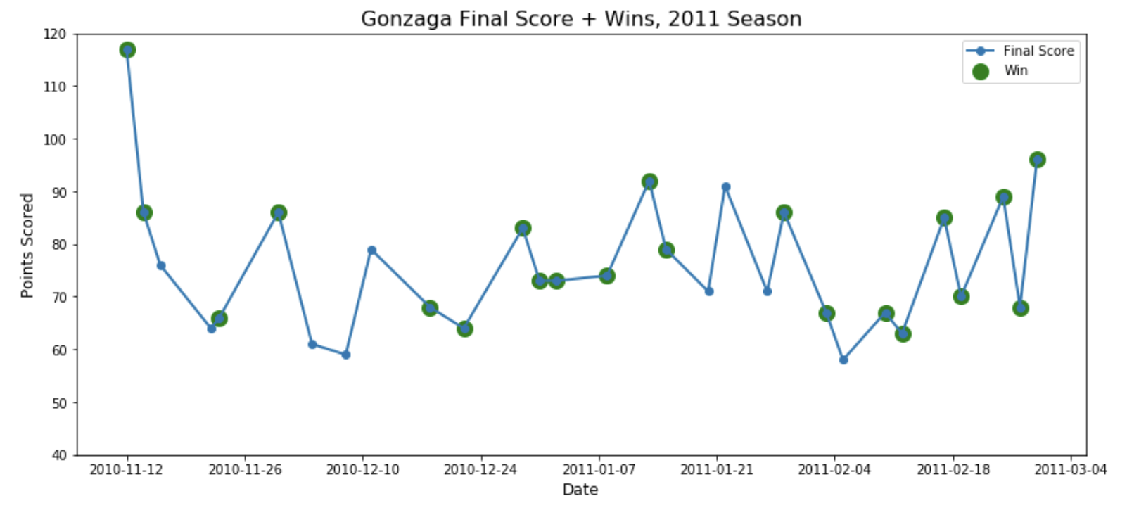
Gonzaga won most, but not all of the games where it scored more points than typical. Conversely, Gonzaga also managed to win a lot of games at the “troughs”, where they scored less points than typical. Teams can manage to pile up wins without necessarily putting up a lot of points.
So I set out to try and best inform my model of four larger charactersistics of any given matchup between Team A and Team B:
- Team A/B’s long-run and short-run winningness/box-scores, independent of opponents
- Team A/B’s long-run and short-run “holding-to”ness, i.e. defensive impact
- Team A/B’s “Strength of Schedule”, a weighting factor to #1 and #2.
- Team A/B’s “SRS”, a Simple-Rating-System score maintained by sports-reference
Long-run metrics aim to characterize how good a team is, historically. I defined this as a 30-day rolling mean to capture approximately a season’s worth of games. It’s equally important to capture short-term variance, due to perhaps player-injuries, or the addition of new talent, so I defined short-run metrics with a few short-sighted exponentially weighted means. This is similarly applied to the alternate team’s “defensive” version of those metrics. All of those previous metrics occur against teams of varying quality, and so I included Strength-of-Schedule (SOS) to inform the model how to appropriately weigh those metrics. Lastly, I included an overall score metric maintained by sports-reference for each individual team.
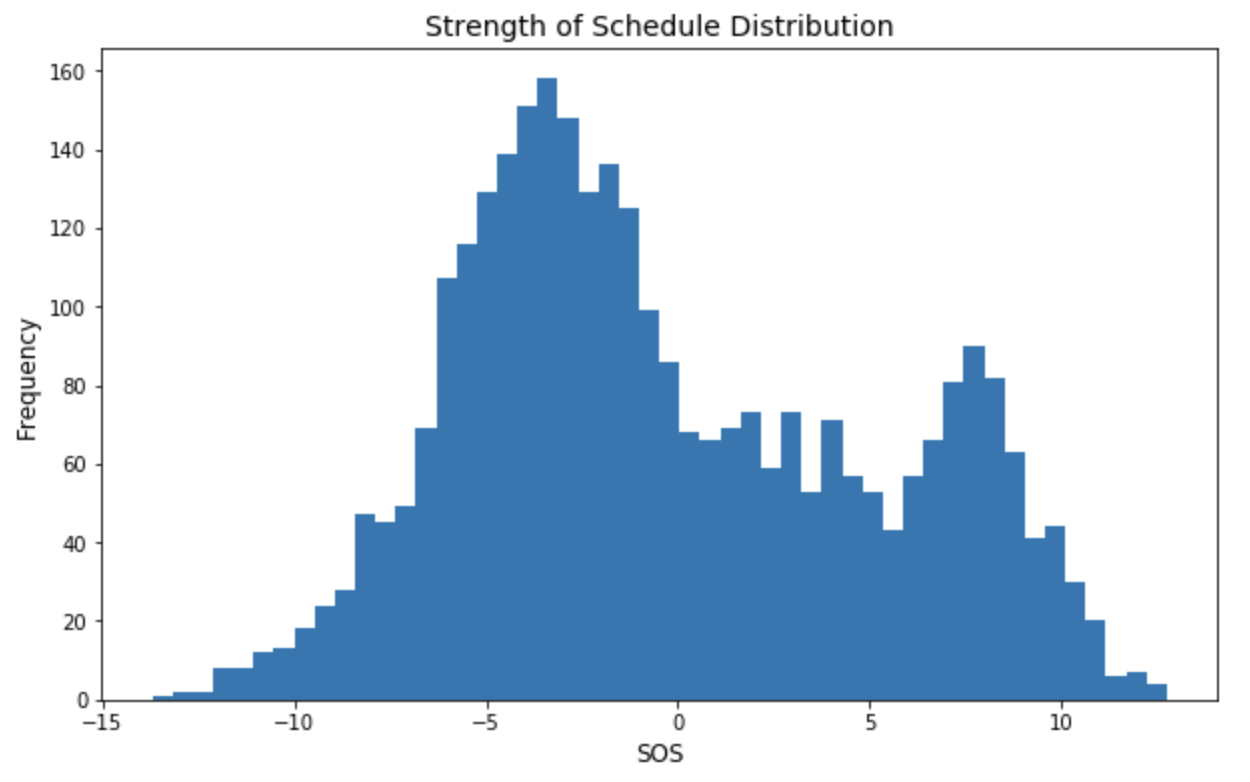
The Strength-of-Schedule histogram appears to have two peaks. This is not surprising, since some conferences are considered much more difficult than others, so there may be “buckets” of teams centered around different values
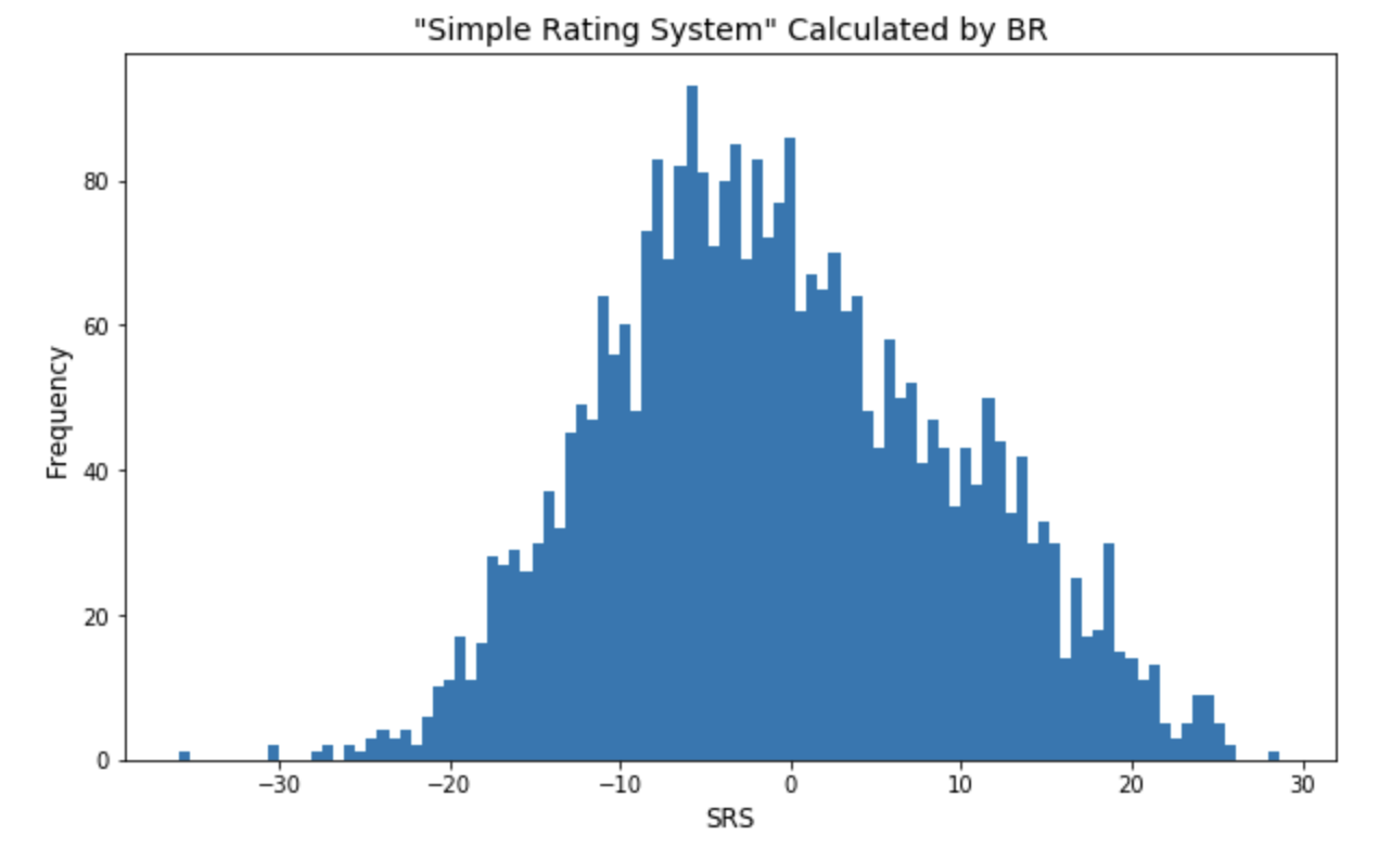
The SRS, determined by sports-reference, is an estimate of how many points a given team would be expected to score over an “average team”. Seeing this histogram centered near 0 is reassuring, since the total summation of these estimates should zero out.
Vegas Accuracy: 74.3%
Since 2003, Vegas Sportsbooks have correctly picked the winning team at a 74.3% clip. See here for history.
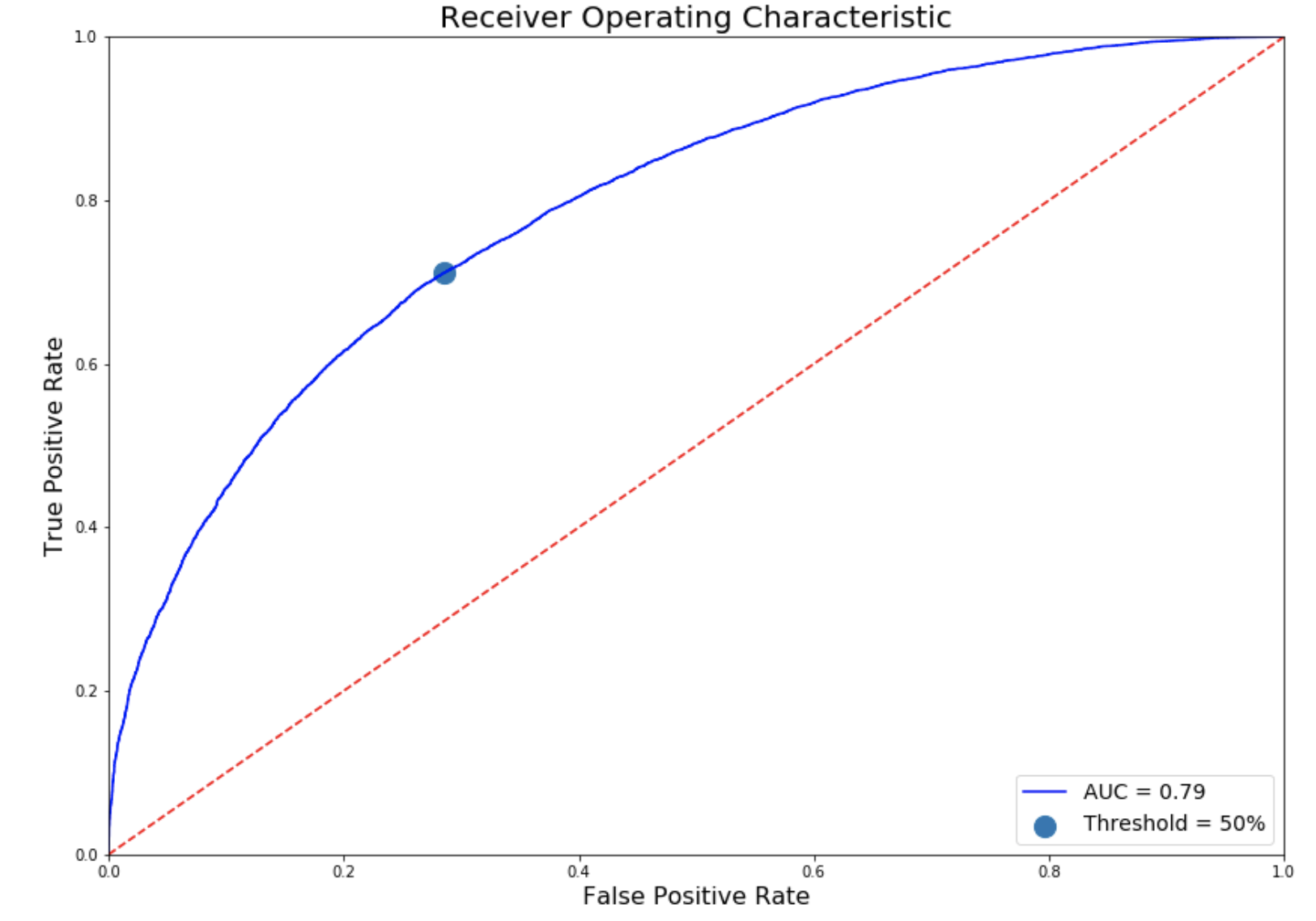
My Accuracy: 72.3%
Hypertuning a Logistic Regression model after conducting Principal Component Analysis to reduce variance, yielded an overall prediction accuracy just 2% shy of Vegas bookmakers. At the 50% threshold, that’s an AUC-ROC of 0.79
Performance vs. “Difficulty”
Logically, we expect the model to perform best in matchups that would be considered “blow-outs”, and worse when teams are considered more evenly matched. Sure enough, that seems to be the case, when we reference the difference in SRS as a measure of “closeness” of matchup:
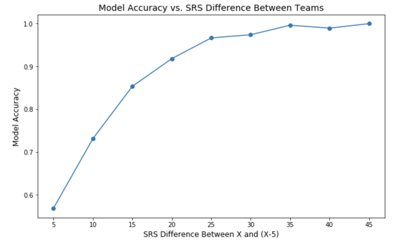
The model performs with over 90% accuracy when there is at least a 20-pt SRS Difference, but drops to 58% when the SRS is within 5 between competing teams. And because conferences are constructed so that more evenly matched teams are often competing, these matchups tend to make up the bulk of regular season games:
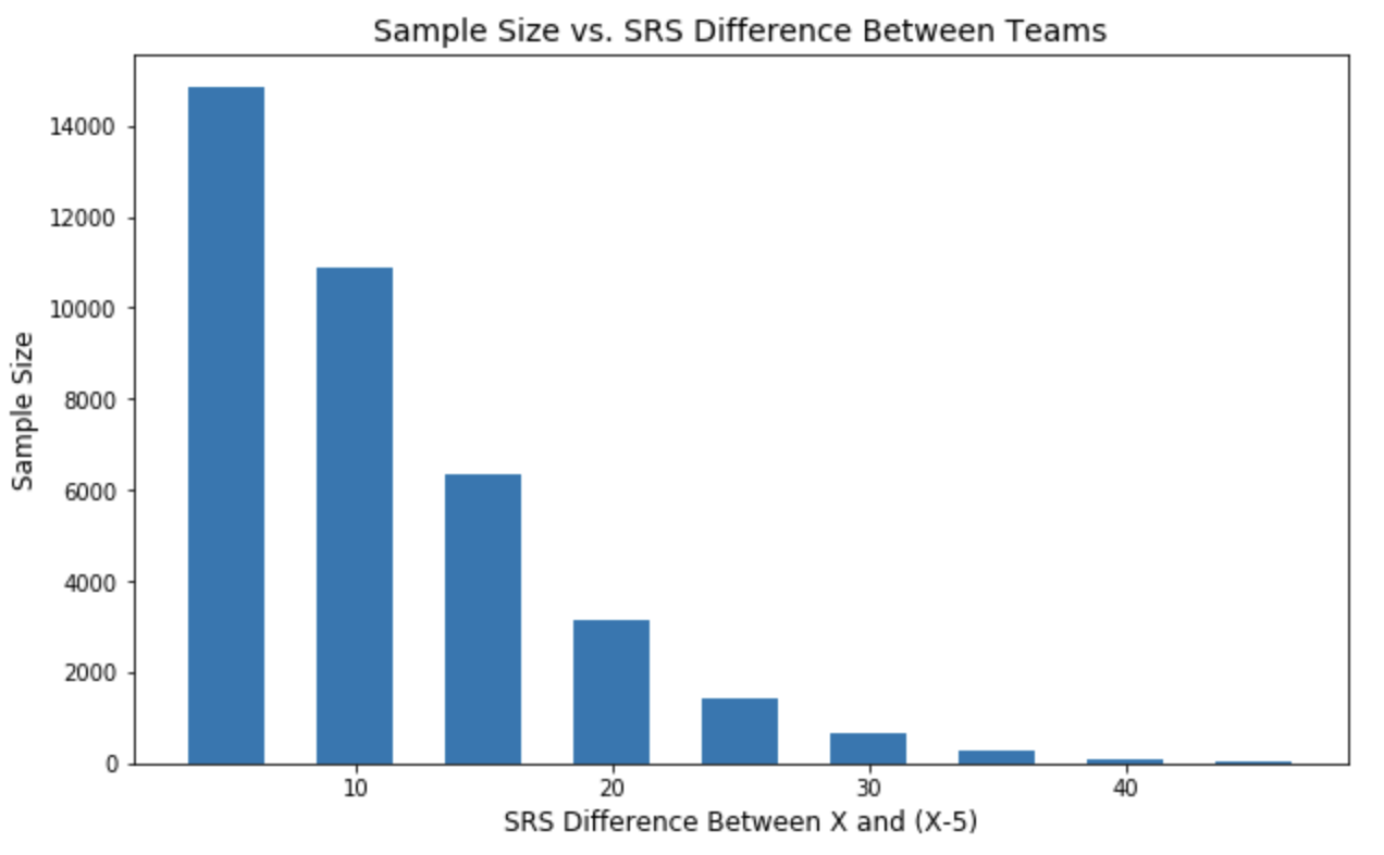
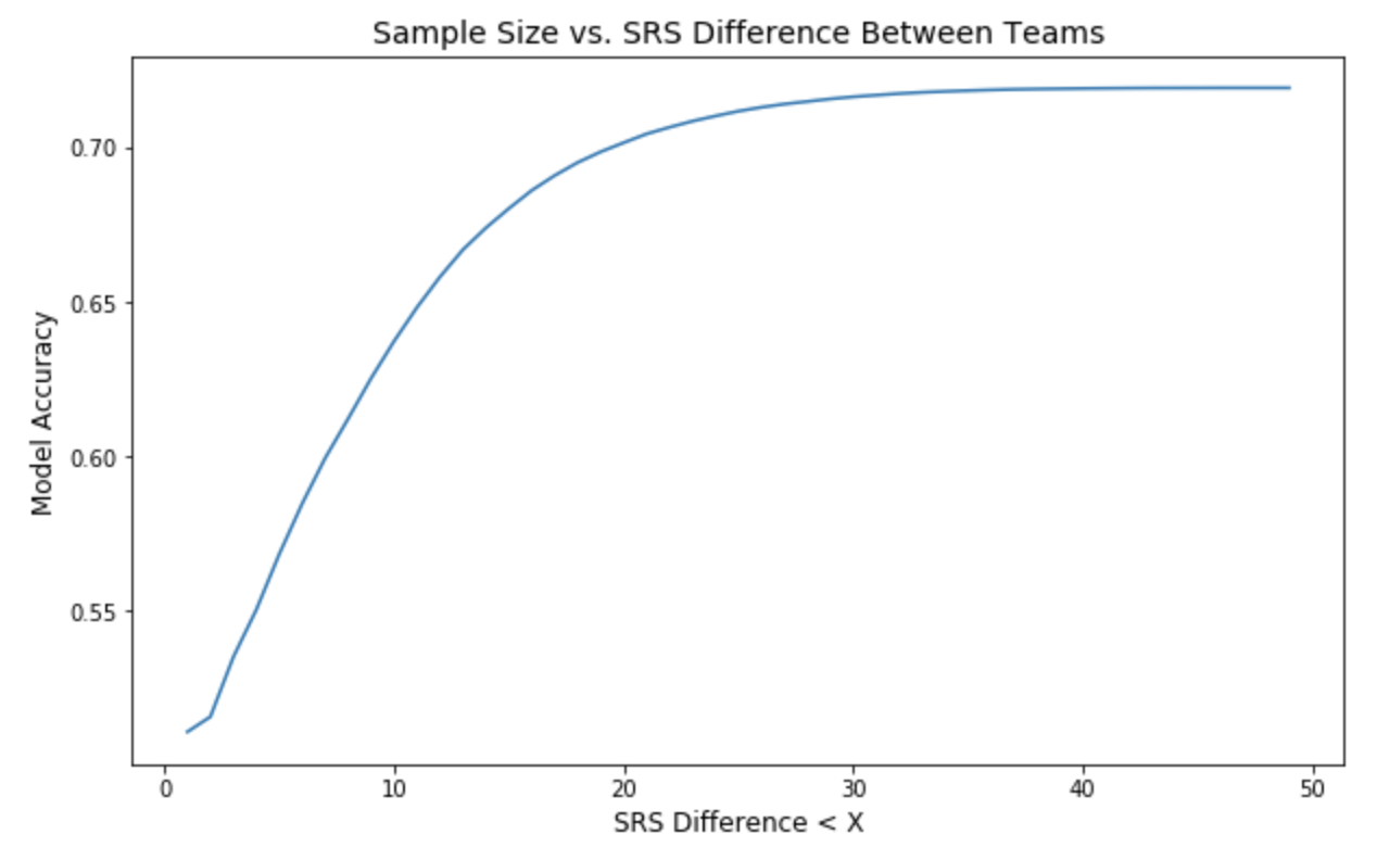
Thus, our model performance aggregately peaks at ~72.4%:
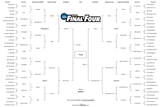
Unleashing the Model on March Madness 2018
Somewhat assuringly, my model heavily sided with the “chalk” picks (selecting the higher-seeded team over the lower-seeded team). This means that my model generally came to the same conclusions as the committees that assigned seeding at the beginning of the tournament. However, a model that only picks chalk isn’t very helpful, so I’ve pointed out the situations where my model tried to predict upsets. (For this excercise, I “reset” my model’s picks at the beginning of each stage so it would always know the two teams that actually ended up playing. In the next section I’ll show how my model did on a “true” bracket).
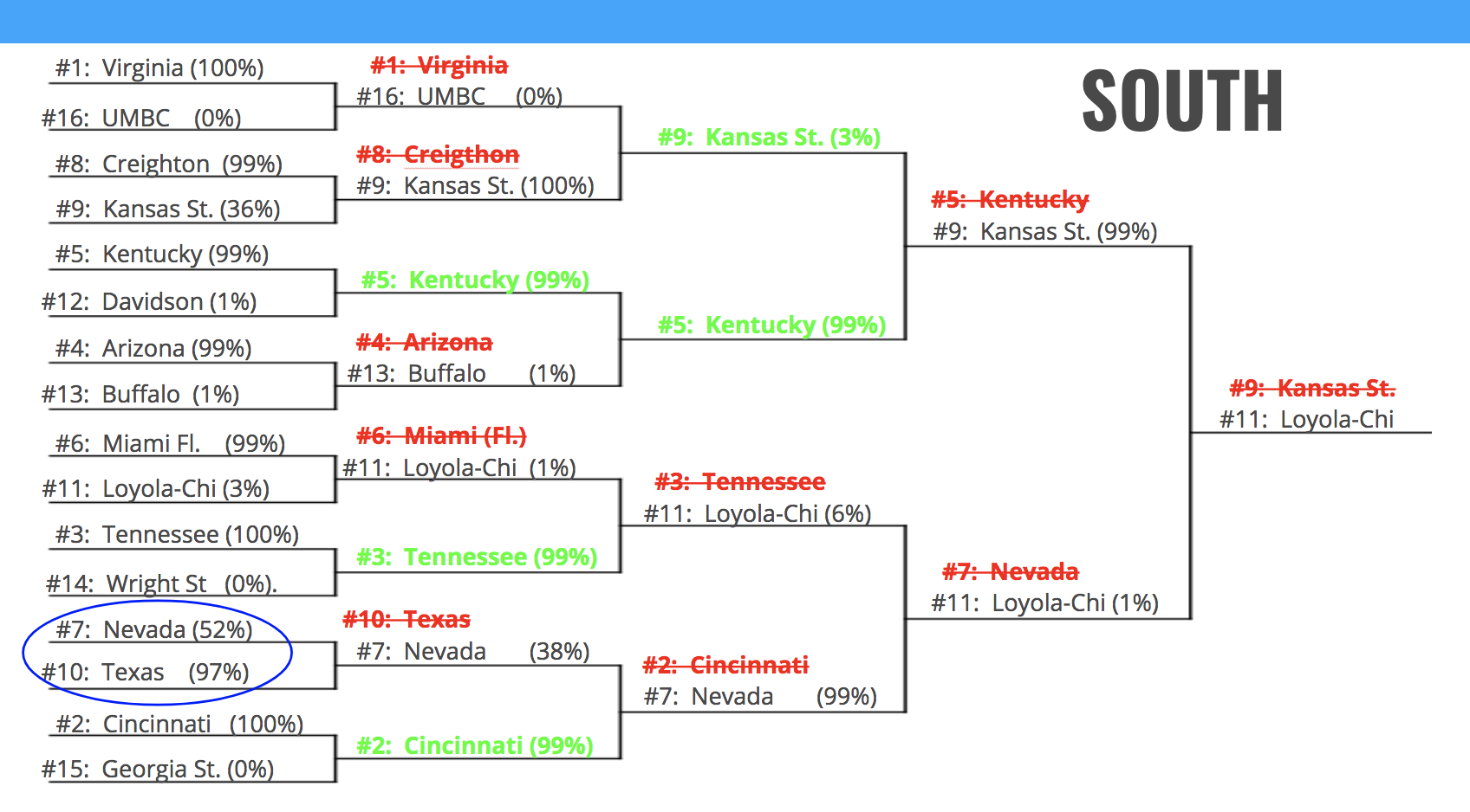
Let’s get the worst conference out of the way first. Here, my model picked all chalk in the first round, with dizzyingly poor results, considering all of the wild upsets that took place (#16 over a #1 for the first time in NCAA history!). The model, did, however try to tease out #10 Texas over #7 Nevada (but unfortunately struck out). The model picked chalk in the remaining stages, with varying results.
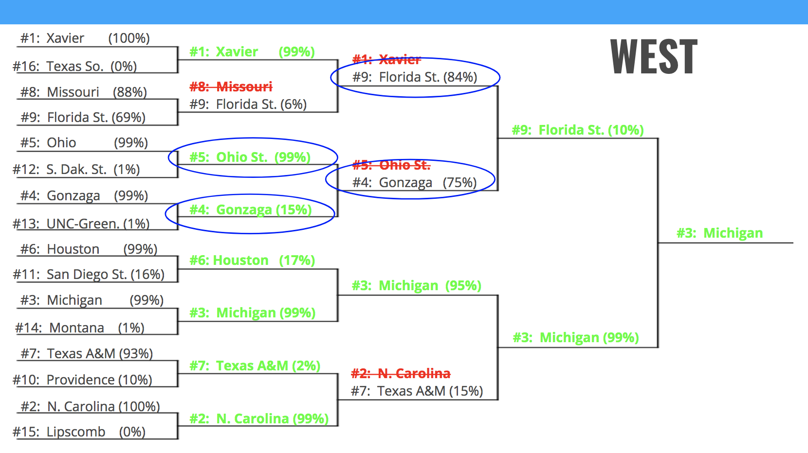
In the West, my model picked chalk for the entire first round, missing only on the #8/#9 matchup (always the most difficult to predict considering closeness of matchup). Interestingly, my model took #5 Ohio over #4 Gonzaga in the 2nd round, but unfortunately struck out on this one, too. However, the model redeemed itself in the 3rd round when it correctly predicted #9 Florida over #4 Gonzaga, a huge upset.
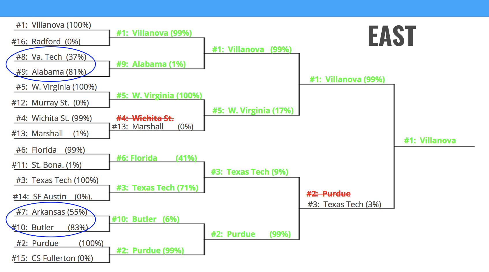
Some great first round news! The model predicted two upsets correctly, #9 over the #8, and #10 over the #7, and only missing one game overall (another, even more surprising upset). The model picked chalk the rest of the way, missing only #3 Purdue over #2 Texas Tech.
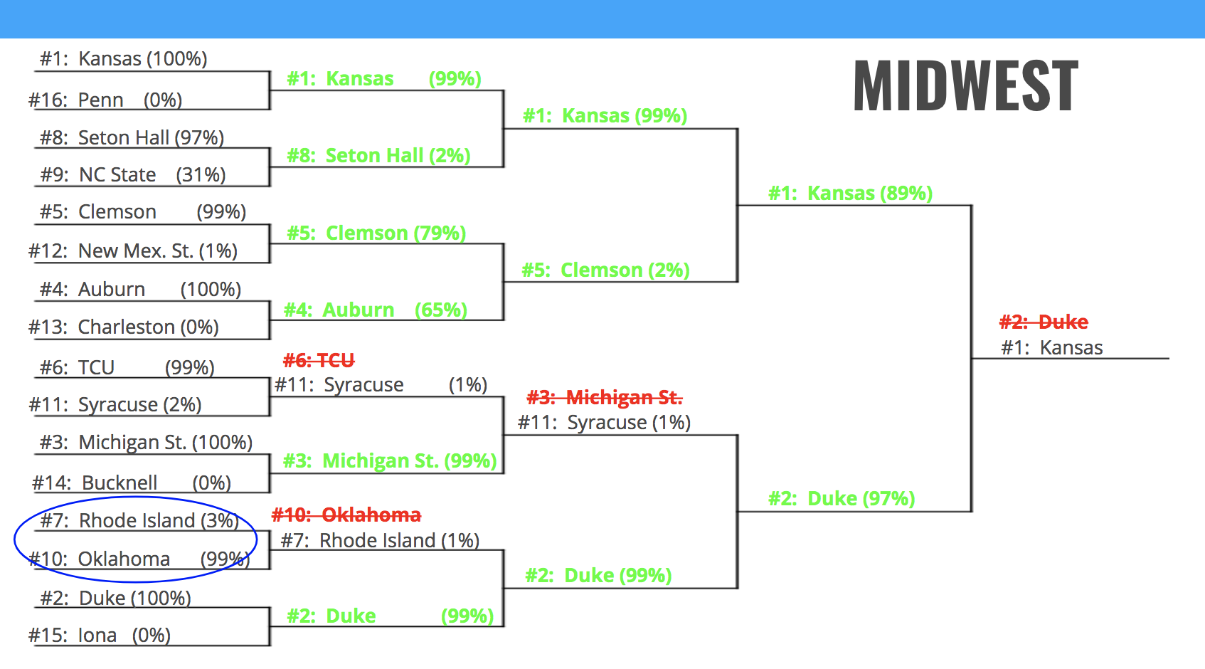
Again, the model tried to tease out a #10 over a #7 in the first round, but missed it. However, it redeemed itself in the 2nd round, correctly picking #5 Clemson over #4 Auburn. It picked chalk again the rest of the way out, with varying results.
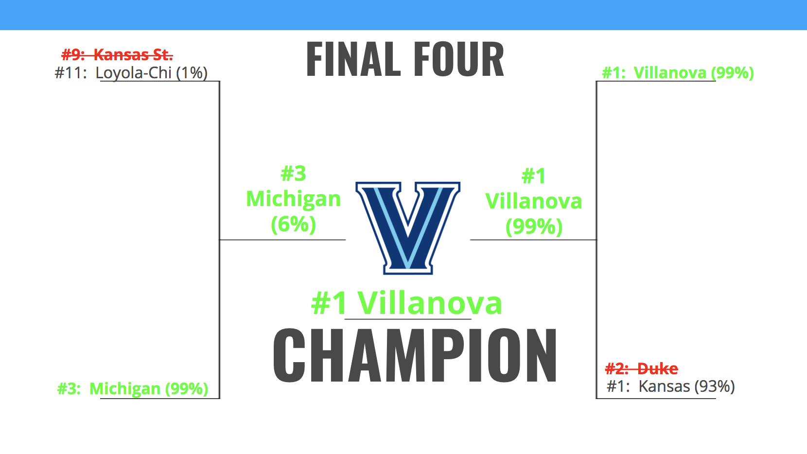
Given the Final Four teams, the model went undefeated. This is not surprising for the #3 Michigan/#11 Loyola-Chi game where Loyola was such a steep underdog, but the #1 Villanova/#1 Kansas and #1 Villanova/#3 Michigan games were considered much more difficult.
If The Model Filled Out an Entire Bracket Before First Tip-off
I’ll spare you the details, but ultimately my model picked a lot of chalk up to the Final 4, and for anyone who followed March Madness this year, higher seeded teams did not live up to their expectations (only 3 #1/#2 teams made it to the Elite 8). But there is a glimmer of hope, in that the model correctly predicted the champion from the outset!
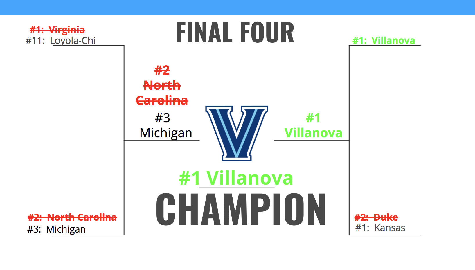
Vegas bookmakers had Virginia/Villanova/Duke as the opening favorites, so I’m excited to see that my model mirrored those predictions, and took it one step further to tease out the winner of those three.
Conclusion
I am definitely pleased with the model’s performance, having approached Vegas bookmaker accuracy. However, 72% prediction accuracy does not translate to very good bracket predictions, since the inaccuracies compound at each stage.
Yet, I think there is still a lot of room for substantial improvement with this model. Firstly, I’d like to include Home/Away designations since Vegas bookmakers have historically assigned an underlying advantages to Home Teams over Away teams.I believe it would also help to include some more granular player information that would be able to identify offensive/defensive player mismatches or exploitations. Team biological information may also provide useful, since it will allow the model to identify when individual team members might have a height/weight/strength advantage/disadvantage over the opponent.
Hope you enjoyed reading, and feel free to reach out with questions or comments! Thanks!